A voltnut, or "metrology enthusiast" as our Brit and DownUnder friends say, is a person who gets really excited about knowing to many decimal places how much voltage and current is running through our little devices. I don’t really need all that, but when I’m playing with digital-to-analog conversion, I do need to know pretty accurately what the real analog voltage is.
I’d like to know to the millivolt, which at 5v means 0.02% accuracy, or "4 1/2 digits," in metrology-speak. Turns out that’s about five times more accurate than anything I have now.
This Fluke was built while I was in college.
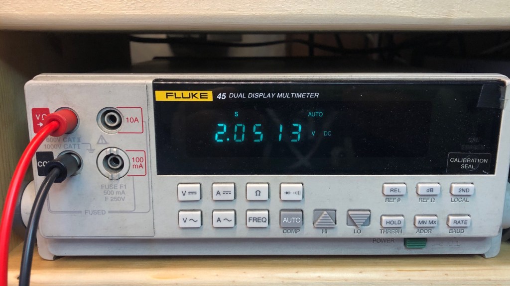
I’ve connected the reference to all threefour of my measurement devices. First I have an ancient but wonderful Fluke 45 multimeter which claims precision to a tenth of a millivolt at the medium reading speed at 3v, or 0.02% (I can’t quite tell from their table). It has a calibration seal dated in December, 2000.
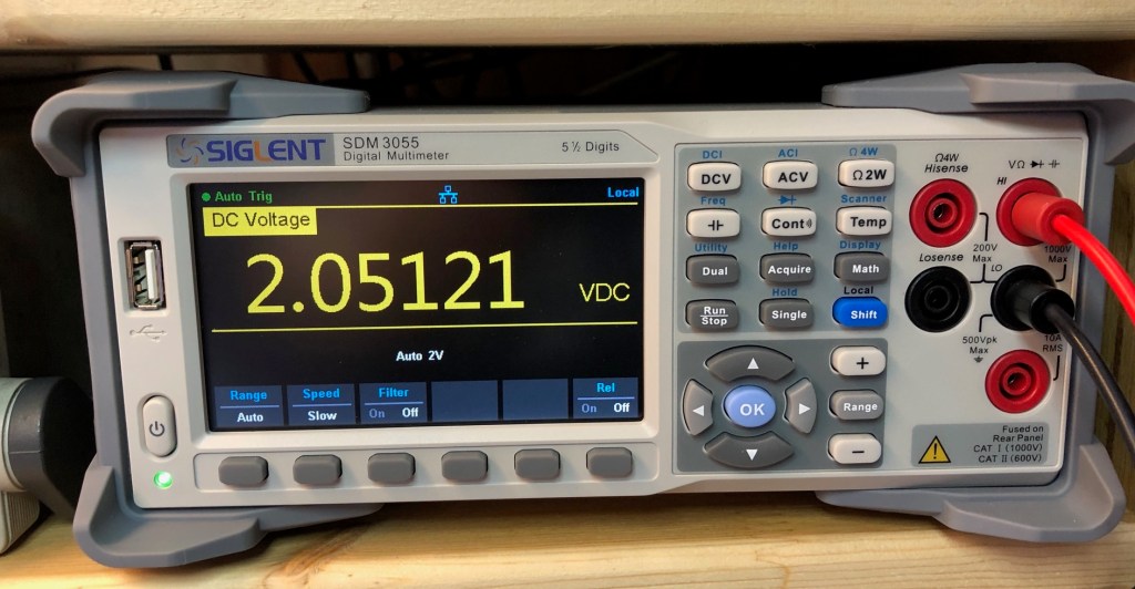
The newest toy on my bench is a Siglent SDM3055 multimeter. I won’t say more about it because mjlorton at YouTube has done a great review. The calibration cert on mine is good thru May 2020.
The Siglent multimeter is gorgeous
Next is my 10-year-old Amprobe 37XR-A, a beefy tool for serious electricians. This beast has been to Burning Man about 8 or so times, but it cleans up nicely for lab work.
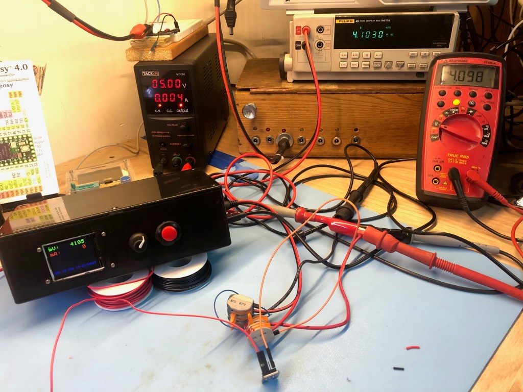
In this test, I’m using Adafruit’s Precision LM4040 Voltage Reference Breakout. I give it about 5v, and it puts out 2.048v or 4.096v at 0.1% accuracy. That means +/- about 2mV and 4mV at the two output voltages, respectively. Setup in the pic below.
Not to put too fine a point on it, I’d like to know which of these devices is the most accurate. Alas, this test doesn’t really tell me. The results are in the table below.
device
2.048v
4.096v
Siglent SDM3055
2.0503
4.1032
Fluke45
2.0506
4.1036
Amprobe 37XR-A
2.047
4.098
ina260 breakout
2.052
4.103
The good news is (i) the calibrated Siglent and the Fluke are indistinguishable at 4.096v, and nearly so at the 2.048v reference (I believe the Siglent). They vary by less than half a millivolt here and in other tests. (ii) The Amprobe and the ina260 are within their tolerances at the 2.048v level, and the Amprobe is still within reference at 4.096.
The ina260 is within it’s stated 1% tolerance, indeed, it’s nearly as good as the other two with better tolerances. This said, it is not a voltmeter: it’s a very delicate IC on a breakout board. Reverse the polarity and you’ll fry the IC, and you can fry an upstream microcontroller’s I2C bus connected to the ina260 board. How do I know this? you wonder.
All this said, I can’t tell from this test which is the most accurate because most of the variation is within the variation on the LM4040. I also bought a AD584 reference, but it produced arbitrary values and seems to be defective.
Three action items emerge: (1) replace the AD584; (2) get the Fluke calibrated. And (3) indulge in a fancy new DMM, which I did. It’s great.
I’m building an r2r ladder which is a way to convert a group of binary voltage inputs to a continuous analog output. For example, an 8-bit r2r ladder would output a single voltage from 0-Vcc at 255 discrete voltage points that are about 20 mV apart.
This is a digital-to-analog conversion (DAC), and I want one in order to build an arbitrary waveform generator (like this one or this one). The DAC will take 8 pins from the arduino, treat them like the bits of a byte, then output a voltage between GND and whatever the Arduino is outputting (Vcc = 3.3 or 5v). That is, we use the DAC to go from a set of digital values in a given waveform to an analog voltage. We need that for any waveform that has a progression from 0-Vcc, such as a sawtooth, a triangle, or a sine.
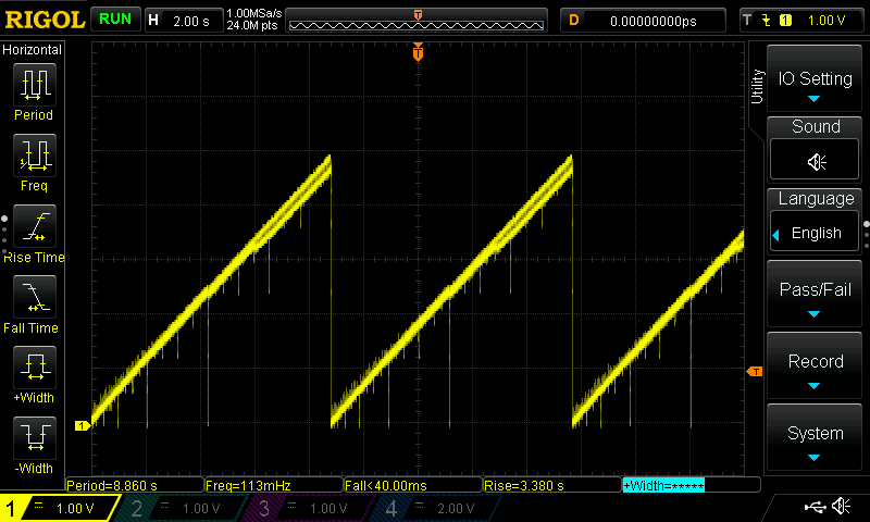
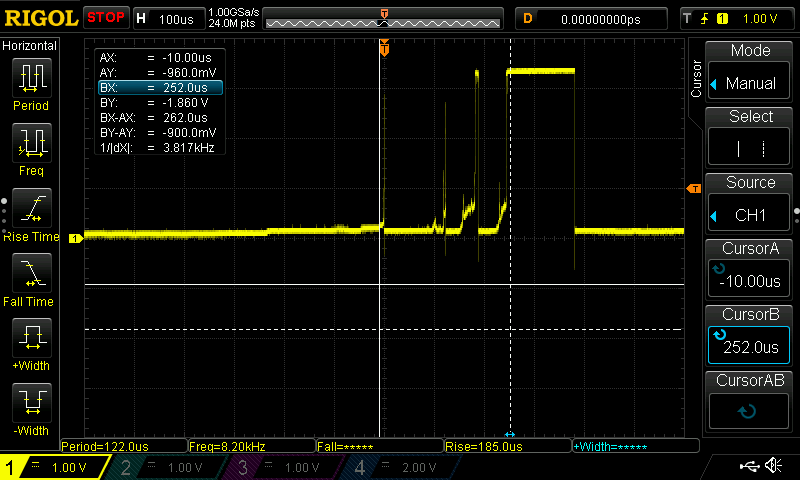
So I built it, added 8 pins from an Arduino, wrote a sketch to step through 0-255 and write the resulting byte to the 8 pins. I measured the result, and it wasn’t quite what I hoped. First, here’s what it looks like on an oscilloscope.
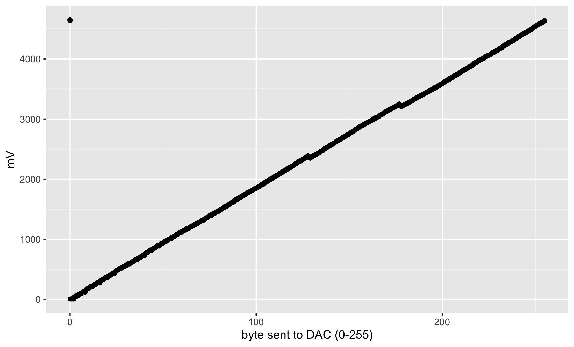
The problem is those occasional big dropouts, the vertical yellow lines that seem to dribble down off the main diagonal. I wrote the data to a file and started analyzing it. First, the voltage-by-byte. I ran over the 0-255 values 30 times to get a decent distribution. It’s not quite the same as the oscilloscope because the ina260 I used to measure the voltage does two things: first, it measures for 140us, which is about 7000 times slower than the oscope. Second, it measures 16 times and then reports the mean of the measures, so in practice, the ina260 is more than 100,000 times slower than the oscope.
This looks mostly good, except for the two notches which turn out to be at 129 and 178. Yikes, and yuck. If we’re concerned about a stable increment between bytes, let’s look at the first differences, that is, (voltage at byte_k) – (voltage at byte_{k-1}). These are called lagged diffs.
As we might expect, the difference clusters around 20mV, which makes plenty of sense. Unfortunately, there’s a second small cluster between -40 and -20. Those turn out to belong to bytes 129 and 174. There’s absolutely nothing interesting about those values, in a binary sense, which is a clue that this isn’t about a wiring error. If the glitches happened at 32 or 64 or 128, that would suggest that I’d done something wrong at a specific resistor.
Looking at the histogram just for 129, 174 there’s also nothing special in the distribution of lagged diffs.
Back to basics: what’s an r2r network anyway? Basically it’s a big voltage divider, and the stability of the output depends on the ratios among the resistances.
The reason we use the r2r pattern is specifically because the combination of 8 voltage dividers in one circuit allows each bit to contribute a unique chunk of voltage to the output. For example, the least significant bit of an 8-bit ladder contributes b/2^8 volts, where b is either 0 (if the bit is 0) or Vcc if the bit is 1. The next-least-significant bit contributes b/2^7 volts, and the one after that contributes b/2^6 volts, etc. The sum of these 8 contributions creates 255 unique voltage values.
That transformation works because in the voltage divider, all the r values are the same, and the 2r values are the same and = 2*r. But unfortunately, that’s not how most resistors really are. The ones I have on hand are 5% tolerances, so r is around 10K, and 2r is in the neighborhood of 20K. I started testing the resistances, and they came in between 9766 and 10055 ohms; the 2r values came in 19789-20129 ohms. These bits of imprecision yield enough weirdness to create the notches and nonlinearities in the graphs above.
Hmm. After a little reading, it became clear that this is how r2r networks fail: inconsistent values, and even more, inconsistent r/2r ratios, lead to nonlinearities –glitches — in the progression of output voltages. This is exactly what I’m seeing. There’s even a Hackaday post about trimming resistors to make them more consistent for this purpose.
I’m not going to do that because I’m lazy. I ordered a few 10K and 20K resistors with 0.1% tolerances from Mouser, and I’ll try again when they arrive.
When you wire a button or a switch into a digital circuit, it might seem as though when the button is pushed, a circuit is closed, and there’s a digital HIGH or 1 available.
It’s not that straightforward, unfortunately. At the microscopic scale, the switch has tiny burrs that connect and disconnect several (or hundreds) times before it settles closed so that current can flow. This is called “bouncing,” and it’s the topic of many really great videos and blogposts. I even wrote one a few years ago, but now I have an oscilloscope so I can dig in a lot more deeply.
Mostly people handle it in software: if you see a button press, ignore everything for (about) the next 100ms, so you only count one press. A similar technique is to poll the button frequently, watching for a series of HIGH values, then counting only once it’s HIGH for a long enough period.
I am going to follow this video and report my findings (also a nice diagram and roundup of simple software techniques in this post). Here’s a picture of what button bouncing looks like.
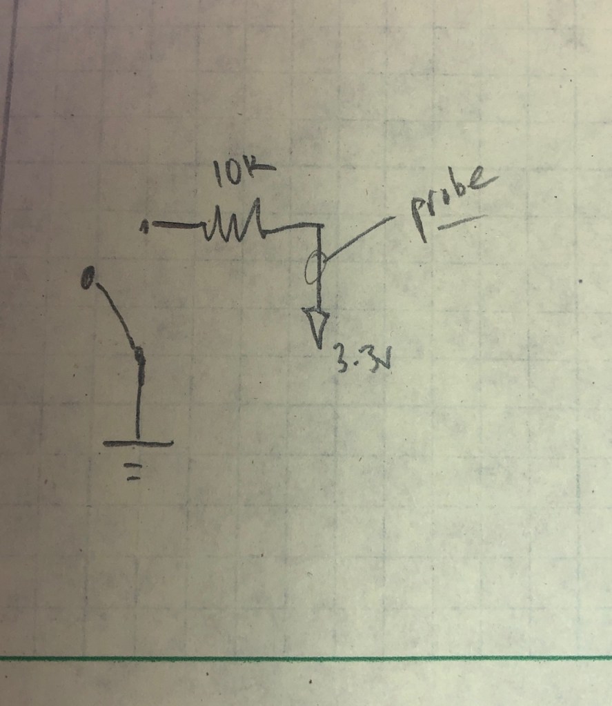
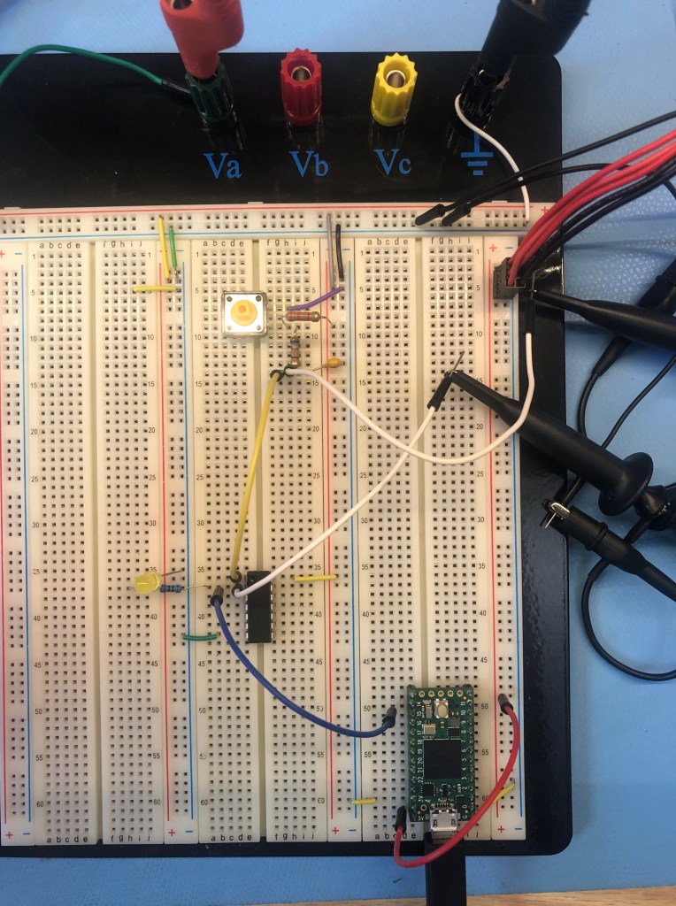
The button is wired on one leg to ground, and on the other leg, through a 10K resistor which connects to 3.3v. The probe is attached to the 3.3v side of the resistor. When I push the button, there’s an initial jump to 3.3 that lasts only about 120 nanoseconds (the solid white vertical line marks when I pushed, and I zoomed in to measure the time of the first bounce). After about 100μs (note that microsecond is abbreviated μs), the contact gets a little closer, and the jumps upward become more insistent. At about 240μs after I pushed the button, the button settles at a HIGH signal (note the dashed vertical line when this happens). I released the button only another 100μs later, and it dropped nicely to LOW (note that there’s not usually much bouncing when a switch opens because all the little rough bits are pulled apart more quickly than when they are closing).
The Teensy 4.0 I’m using here runs at 600MHz, about 6 cycles/μs. So there are more than 1500 cycles during the 262μs this button is bouncing. It’s easily capable of counting the 8-10 bounces above 1.8v (where it counts HIGH). That creates a mess when you’re trying to count button pushes.
For my test, I’m doing 2 separate things to the signal. First, I smooth the bouncing using a resistor-capacitor (RC) circuit. I can’t explain RC circuits, that’s a bit above my skills so far, but I recommend the Art of Electronics Lab Course, chapter 2. I’m digging through it now.
When the switch closes, the capacitor discharges according to the time constant, τ = R x C. The idea is that it takes about 5τ for the RC circuit to charge or discharge. The charging is exponential, not linear, and there’s a great tutorial about it here but alas, the graphics seem to be missing.
My graphics aren’t great, but here they are. R1 is the pullup resistor, and it’s 2K. The RC circuit starts with R2 at 680Ω and the capacitor is 1μF. That means that τ = 6.8e-4 secs, so it charges or discharges in 5τ = 3.4ms.
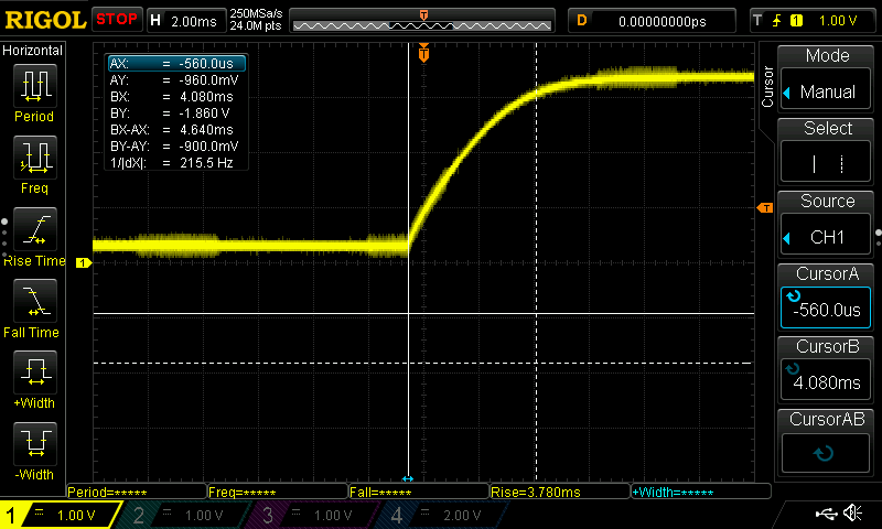
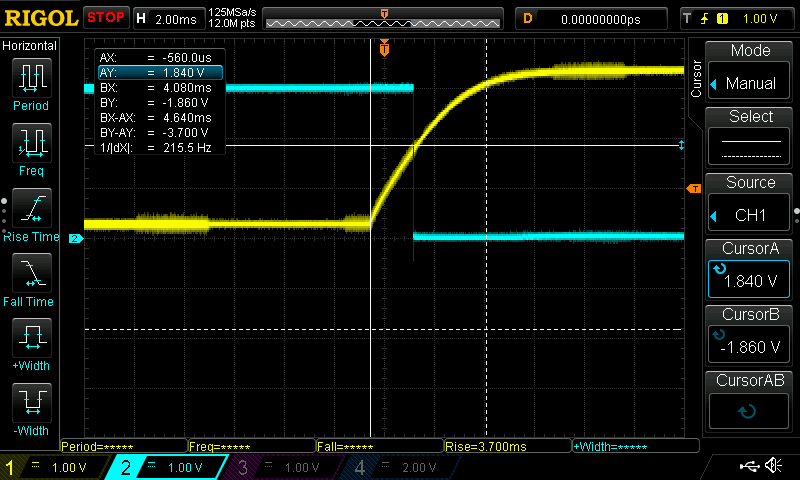
This is what happens when I press the button and measure the signal in parallel with the RC (before IC1 in the schematic above). Note that the two vertical lines mark the beginning and end of the capacitor’s discharge. BX-AX is about 4.6ms, which is pretty close to the theoretical 5τ = 3.4ms. I’m happy when my experiments match theory.
The point of this is to get a digital signal to the microprocessor, but the RC signal isn’t really square, it’s curved which forces the microprocessor to decide when the signal is HIGH. The Teensy can do that, of course, but once we start building this circuit, shouldn’t we get a square signal out of it?
The answer is an inverting Schmitt trigger, an integrated circuit that shifts from 1 to 0 at some higher threshold, and from 0 to 1 at a lower threshold. It’s an inverting trigger, which means that it’s output is always the opposite of the input, as seen in the image above. The yellow line is from the RC circuit which is the input to the trigger. For the trigger, I’m using a 74HC14, an integrated circuit (i.e., a chip) which switches from high to low when the input voltage hits about 1.8v (when the input voltage to the chip is 3.3v).
Note that as the yellow line gently climbs, when it hits 1.8 volts, BAM, the Schmitt trigger output shown by the blue line drops from HIGH to LOW. The datasheet reports that the drop happens in about 7-19ns; My oscilloscope sees the transition in 14.8ns: good job, datasheet. By comparison, the CPU on the Teensy is running at 600mHz, which means about one cycle takes 1/600th of a million-th of a second, which is approximately 2 nanoseconds. While it only takes one cycle to read the digital pin (in the very best case, usually it’s more), the Arduino is doing other stuff and can’t check the pin every cycle, so it won’t read the pin more than every 50-100 ns. The Schmitt trigger switches in about 15ns, 8x slower than the CPU. There’s very little chance chance that the Teensy will be confused during the trigger’s transition.
Here’s what it looks like wired.
The code that runs the counter is below. I’ve banged on this button something fierce, and it counts once and only once every time I hit it. There’s no software debouncing at all, the hardware is doing all the work.
I like it! It’s pretty unnecessary: I’ve found that a simple delay works for nearly all my applications, and in exceptional cases like rotary encoders, state machines work a treat. However, I’m really happy to have had a reason to look more deeply into this topic and to have another tool in my kit if a switch acts up.
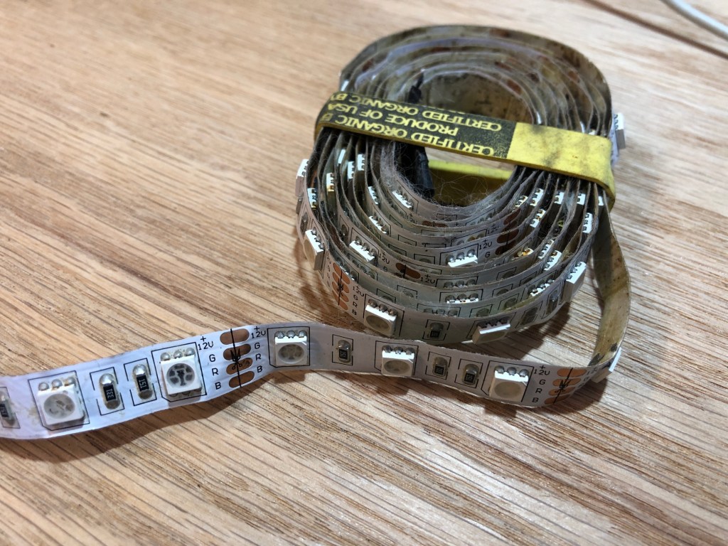
My friend Bear was on the BM cleanup crew this year, and he came upon a seriously tricked-out bike that had been abandoned, locked to a bike rack at a big sound camp. He removed the electronics for me to study. There are 8 strands of analog (not individually-addressed) 12v RGB LEDs, like this one.
So 8 * 3 (RGB) connections (each of which sinks) is a quick tip here. Of course there’s an Arduino.
Then it gets more interesting for me. The Arduino sends a serial signal to a series of 3 74HC595N shift registers, thereby splitting the serial signal into 24 (ahem, 8 * 3) parallel 5v outputs.
But the LEDs are 12v, and will need to sink a lot of current. Here’s where the lost inventor does something I would not have thought of: they used 3 ULN2803AN ICs to sink a lot of current (again 24 signals, but at 12v!), switched by the Arduino at 3.3v.
Note that the ULN2803ANs are stacked, one on top of another, putting them in parallel so each output can sink up to 1A. Good thinking, and careful soldering.
There’s a lot for me to learn with this teardown. Using the ULN2803AN as an array of Darlington transistors is pretty cool. I’ve used single Darlingtons before, and it seems that arrays of transistors and resistors is something I’m learning about right now (more on this in a later post).
Even more, the inventor has srsly used perf board before. They organized the chips and the headers to minimize the wiring in smart ways that I’m going to keep studying.
It sure is great to have a lab to study stuff like this! Thx to Bear for spotting this in the dust and schlepping it home for me.
But not quite yet, there are a few things that will need doing first. So in the meantime, I want to recognize two artists whose work I find inspiring and absolutely mind blowing.
First, Hedeki Inaba is off the hook. His new piece with musicians Canigou, called Tape is so great, just, wow. This is a great way to represent how I experience writing and thinking about software, synesthesically speaking.
Second, Naoto Hattori is incredible. His work is whimsical, adorable, and completely nuts. I feel like this is the next step on adorable cat pix. This piece is characteristic.
Burning Man is trying to get a ten-year agreement to continue holding the event in the Black Rock Desert. The Bureau of Land Management (BLM) has done a farcical Draft Environmental Impact Statement. Burning Man has analyzed the DEIS, and is calling for Burners to write comments. Cory Doctorow has written a terrific model letter.
I’m not going to repeat all the nonsense, but I’m pasting my letter below. Sheesh. C’mon folks, buckle down and write a letter. This is some serious bullshit.
———- Forwarded message ——— From: Me Date: Sun, Apr 7, 2019 at 5:32 PM Subject: environmental impact statement for Burning Man To: <blm_nv_burningmaneis@blm.gov> Cc: <eis@burningman.org>
Dear BLM,
I have read an overview of the Burning Man DEIS with particular attention to the recommended mitigations. I have three comments and associated questions based on my ten years attending Burning Man.
First, the call to increase security by requiring Burning Man to contract a private security service (PHS-1) is unnecessary and unjustified by the evidence presented. The “screening” foreseen in this claim is a search that is patently unconstitutional under the Fourth Amendment. The National Environmental Policy Act cannot be lawfully stretched to cover surveillance of this sort. It is grossly improper for BLM to request it.
The additional time required for the proposed screening of participants at the gate would be burdensome to the public and harmful to the environment. To be clear, Black Rock City is already pretty safe: in ten years I’ve had no issues whatsoever with firearms or anything else that required law enforcement. Indeed, the most serious safety risks I see each year are inevitably BLM Rangers and other law enforcement officials who are driving too fast.
Nearly every year I have to file notices with the Burning Man Rangers about unsafe driving by law enforcement; in 2018, I filed three notices. This happens both outside the city and inside the city when law enforcement speeds by pedestrians and bicyclists. The consistently irresponsible driving of BLM Rangers and Nevada county sheriffs also affects mitigation AQ-1. Just a few hours of observation out there makes clear that law enforcement vehicles speeding at well over 30 mph through unfenced areas are among biggest creators of dust problems.
What measures have you put in place to oversee the BLM Rangers to assure that they respect the safety and constitutional rights of the participants? I’m not asking that BLM Rangers “protect” participants’ safety. To the contrary, and to be clear, my question is: what is BLM doing to make sure that BLM Rangers don’t imperil people by unsafe driving or by unnecessary and violent policing? What training do the Rangers receive in protecting participants’ rights?
Second, the jersey barriers (PHS-3) are unnecessary. There are very few people who attempt to gain unauthorized entry into the event, and they are swiftly caught by Burning Man’s Gate, Perimeter, and Exodus staff. Have you considered how much energy would be required to manufacture and transport *nine miles* of jersey barriers? That’s about 19 million pounds of concrete and steel, perhaps one thousand 100+ mile round-trips in a flatbed semi trailer from Sparks or Reno. Have you done the environmental impact analysis on this “mitigation?”
Third, the additional fluids (WHS-4) and wastewater (WHS-6) requirements are similarly unnecessary. I’ve built a number state-of-the-art “evapotron” towers to that eliminate about 200 gallons of greywater per week per tower, without leaking and without waste on the playa. Our evapotrons are regularly admired by the Earth Guardians. Consequently I’ve spent a lot of time over the years helping Burners capture, evaporate, and transport their greywater — and they’re pretty good at it. As a Burning Man greywater guru, I believe that your analysis is substantially in error.
To close, this Draft EIS seems to me a trumped-up list of invented problems. Burning Man has shown itself to be an extraordinarily good steward of public lands, bringing tens of thousands of people to a remote location, year after year, with an admirable health and safety record, while leaving no trace. The Draft EIS ignores this history.
I look forward to receiving your plans for BLM Ranger retraining, an impact assessment of manufacturing and transporting 19 million pounds of steel and concrete, and an evidence-based, statistically rigorous analysis of the DEIS’s wastewater claims.
My big archiving project is slow. It’s hard to iterate on solutions when each meaningful test can take 10+ hours, and in some cases, multiple days.
The most important bottleneck in the process is reading and writing to disks: this task is io-bound. The table below shows the read and write speeds according to the Blackmagic speed test. All tests are run in MacOS 10.14.
disk & interface
read
write
type
interface
MBP2018-internal
2533MB/s
2675MB/s
ssd
nvm-e
archives-2019
82MB/s
86MB/s
5400
usb-c
photos
80MB/s
88MB/s
ssd (samsung T5)
usb-c
archives-2018
81MB/s
86MB/s
5400
usb 3.1
MBP2013-internal
400MB/s
459MB/s
ssd
sata
GDrive ext
189MB/s
187MB/s
7200
tbolt2+RAID1
GDrive ext
184MB/s
173MB/s
7200
usb-c/3.0
The external speeds are consistent across both machines, and this test shows the very best case. In real-world copying, the speed falls to extremely slow speeds — sometimes less than 1MB/s — which I attribute to a combination of lots of hardlinks (see below) and in some directories, hundreds of thousands of tiny files. I’m working on these latter two questions, but still, these raw, best-case speeds seem to me inadequate. I’m not sure why these disks are so slow.
Update: I think the limiting factor is input/output operations per second (IOPS, or reported as tps in iostat). This wikipedia article suggests that spinny disks (as opposed to SSD disks) can sustain 100-200 IOPS/s. Finding a specific sector where a file is is one IOPS, so this effectively limits a disk to reading 100-200 files/s, even if the files are very small. This is really slow when there are millions of files. SSD disks are ridiculously better at this kind of task.
That said, my 500GB Samsung T5 isn’t doing any better at the Blackmagic test, so I’m still a little vague about what’s going on.
In re hardlinks: When I’m copying, I’m using something like rsync -rtlOWSH which copies hard-linked files as hard links on the destination filesystem. rsync has a tough time with hardlinks because it needs to keep a table of all the inodes it has seen during the run. Even as rsync eats up RAM, it is slowing down. I am writing a copy-by-inode tool to work around this problem.
One of the steps in my massive file-archiving project requires that I save all the paths with their associated inodes and sizes from each filesystem I intend to integrate. I’ve decided to save the info to a sqlite database (the link has a great tutorial: if you already know how to use SQL but need the specific sqlite idioms, this is a great page).
The table below shows several approaches to getting the filesystem data into the database. I’ll list the winning command here, then explain the alternatives:
This is gnu find, I’m not sure if the BSD find that ships with MacOS has the same options. You can install gnu find with homebrew, and this link shows you how to use the default name (i.e., find rather than homebrew’s gfind) to override the BSD find.
Anyway, find prints a pipe-delimited list of path, inode, and size to stdout; pv writes a nice progress message; and then sqlite imports directly from stdin. Note that you need to create the table (paths) before this step.
test
speed
comment
base
0.01s
just setup
find | sqlite
0.17s
very simple
find->tmp; sqlite import
0.26s
not as clean but simple
find->tmp; python+sqlite import
0.22s
python buffers better?
os.walk over dirs +sqlite import
0.35s
find is much faster
This table shows results on a test directory of about 21G including about 30K files. The find-piped to-sqlite is considerably faster than the other options: it’s slower to redirect find to a temporary file, then import it; it’s a little better to have python read the temporary file then insert the values into sqlite (I think python parses the file faster than sqlite’s import does: I’m using pandas to parse the file); and then using python’s os.walk instead of find is much slower.
My guess is that the find | sqlite option benefits from a bit of concurrency and smart buffering. The shell (zsh, in this case) is getting a chunk of data from find and passing it to sqlite, letting find run while sqlite does the import. On a much bigger directory, I can see both find and sqlite using CPU time. Eventually everything slows to the speed of the slowest process, but the buffer is big and both can happen mostly at once.
This is a big help for my coming tool which is a mass file-copy script that doesn’t choke on tons of hardlinks (which cp and rsync most definitely do).
Among the files I want to organize in this giant archiving project are photos. These could be scanned images of old paper photos, jpgs from my phone or shared with me, or jpgs and raw files from a couple of decades of electronic photography.
The problem is that the files are scattered across backup systems that go back decades. To collect all the images, I wrote a little python script called getpix.py. (Note that the filename is a hyperlink to the GitHub gist which I’m double-linking because wordpress doesn’t format a code literal+hyperlink in an intuitive way).
Anyway: the script recursively descends a source directory and moves every image it finds to a destination directory in the format bydate/YYYY/MM/DD.
At every directory, the script runs exiv2 on every file (this could be improved by making the subprocess call to find smarter). Files that have a timestamp use it for the directory sorting. If not, and there’s a timestamp in the path (which Apple photo directories often keep), that timestamp will be used. One could add a final fallback date to the file ctime, but at least for me, the file metadata is so badly mangled that it provokes more confusion than enlightenment.
Files with no dates are sorted into no_date.
The resulting bydate structure can be dragged into the rest of the archiving process. There will be lots and lots and lots of duplicate images, and this is a gigantic PITA. There is a Right Way To Do It: use PhotoSweeper. This app will review all the images, link duplicates, and delete extras using configurable and intelligent defaults.
Note to self: do not try to do this inside Lightroom, what a mess that is.
I’m left with about 30K images, which Lightroom can handle without even turning on the CPU fan. This is a step forward.
I have a lot of data from a lot of years: about 5TB with around 8 million files. It’s very redundant, lots of copies of the same stuff. Many of the files are tiny, e.g., 100,000 1-2KB files in Maildir.
Most of the data are now on medium-sized external disks (2-8TB each) accessed via USB or Thunderbolt. It’s time to get everything onto a small set of usable disks (I’ve tried this before and I didn’t get very far).
One of the things that slows me down is that no matter how I set up the copy (cp, rsync, Finder), after a few minutes, the copy slows to a crawl. These are reasonably fast disks on USB3.0 or Thunderbolt2.0. The r/w speed on the disk should be around 150MB/s, and the connection is 5Gb/s, but I’d often see read speeds around 0.5MB/s. Ooof. You’re not going to move a terabyte at that speed.
And now I think I know what’s happening: the directories get disorganized. I am frustrated that I can’t figure out what this means, but I discovered that after running DiskWarrior on the offending drive, it’s now copying at 50-100MB/s (I’m using iostat to watch the r/w speeds). A big, big win.
Of course, APFS makes this useful knowledge nearly obsolete. Ah, the story of my life, learning useful stuff just as it becomes a kind of vintage affectation.
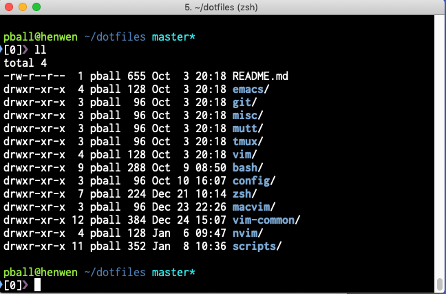
Gotta go, I’m going to write some shell scripts to make my terminal prompt look cool.